Data Science in Astronomy: Clustering

In astronomy, the term "clustering" typically implies galaxies being clustered and refers to their distributions not being uniform random but coupled to the dark matter. In data science the term is more general, referring to the task of breaking up a data set in groups of samples that are more similar to others in the same group than to those from another group. Replace "group" with "cluster" and you have an operation definition of what clustering attempts to do.

To make the most of the terminology clash, we'll use an example of DES red-sequence galaxies in field of several galaxy clusters. That is to say that by virtue of the selection, these galaxies are strongly clustered, but the field is complex, with overlapping clusters of various shapes and magnitude. As we'll see, that's not a trivial problem for data clustering.

# load the data
import numpy as np
from sklearn.cluster import KMeans, MeanShift

data = np.load('clusters.npy')
print (len(data),data.dtype.names)

%matplotlib inline
import matplotlib
import matplotlib.pyplot as plt

# tangent plane to the sky
ra0, dec0 = data['RA'].mean(), data['DEC'].mean()
X = np.dstack(((ra0-data['RA'])*np.cos(data['DEC']*np.pi/180), data['DEC']-dec0))[0]

fig = plt.figure()
ax = fig.add_subplot(111, aspect='equal')
ax.scatter(X[:,0], X[:,1], alpha=0.1)
ax.set_xlabel('$\Delta$RA [deg]')
ax.set_ylabel('$\Delta$Dec [deg]')

1107 ('MEM_MATCH_ID', 'Z', 'RA', 'DEC')

K-means algorithm

The go-to clustering algorithm. It uses $K$ clusters and optimizes their means (duh!). In detail, it starts with $K$ cluster center positions $\mu_k$ randomly placed over the data volume, and then it repeats two steps until convergence: * Cluster asignment: for each sample $i$, add it to cluster set $C_k$ with the nearest mean according to $\text{argmin}_k \lVert x_i - \mu_k\rVert_2^2$. * Recompute mean: for every cluster $k$, update $\mu_k\leftarrow \frac{1}{|C_k|}\sum_{i\in C_k} x_i$.

This sequence consitutes an EM prodcedure (we've come across it before in the Gaussian Mixture Model) that minimizes the sum of the total dispersion $\sum_k \sum_i \lVert x_i - \mu_k\rVert_2^2$. Even on closer inspection, it share a lot of similarity to the GMM. In fact, it can be considered a very limited form of the GMM, in which the cluster assignment is hard (first step) and only the means are optimized (second step). In the full GMM, one has fractional assignments $q_{ik}$ of sample $i$ to cluster $k$ and updates amplitudes, means, and covariances of each Gaussian components.

From this insight, we can already see what character the $K$-means clustering will have. * It doesn't like overlap (hard assignment) * It likes clusters with equal magnitude (no amplitude adjustment) and equal size (no covariance adjustment) * It prefers clusters to be round because the only metric is spherically symmetric and there's no cluster covariance that could change that.

However, because it does so little, it's pretty fast and generally gives a decent first shot at many clustering problems. Let's see what it can do.

Note: We assumed to know the cluster number $K$. There's no inherent way the algorithm could decide for itself what that number should be. Below we'll like into ways of avoiding that decision, but for now we'll have to choose this as users.

for K in range(3,30,5):
    clf = KMeans(n_clusters=K)
    labels = clf.fit_predict(X)
    centers = clf.cluster_centers_
    fig = plt.figure()
    ax = fig.add_subplot(111, aspect='equal')
    ax.scatter(X[:,0], X[:,1], c=labels, alpha=0.1, cmap='Paired')
    ax.scatter(centers[:,0], centers[:,1], c=np.arange(1,K+1), s=1000, marker='+', cmap='Paired')
    ax.text(0.05, 0.95, 'K=%d' % K, va='top', transform=ax.transAxes)
    fig.tight_layout()

As expected, we see plausible results, but in detail, there are flaws: At larger $K$, the algorithm prefers to break up bigger clusters in smaller ones before breaking up smaller, but really fragmented ones (no amplitude variation) and breaks bigger clusters along the semimajor axis (sphericity kicks in).

But the fundamental question remains: can we find the optimal cluster number $K$?

Alternatively, can we avoid the decision altogether? Enter the ...

Mean-Shift algorithm

Where K-means is related to the GMM, Mean-Shift uses a KDE internally to construct a smoothed density distribution $\hat{f}_h$ of the samples. It then throws down test particles at many locations $y_j$ and advances their positions along the local gradient of the smoothed density $$y_j \leftarrow \frac{\sum_i x_i g\left(\frac{\lVert x_i - y_j\rVert}{h}\right)}{\sum_i g\left(\frac{\lVert x_i - y_j\rVert}{h}\right)},$$ where $g$ is a suitable kernel function and $h$ is its bandwidth. With a little algebra, we find that mean shift $$m_j = y_j^{\mathrm{it}+1} - y_j^\mathrm{it} \propto \frac{\nabla \hat{f}_h}{\hat{f}_h},$$ i.e. the test particles walk uphill with a step size that is set by the inverse local density $1/\hat{f}$. In other words, the will quickly move out of low-density areas and converge (provably, in fact) and the modes of the smoothed density distribution.

This is where the next step kicks in: if the test particles overlap within some fraction of the kernel bandwidth, they will be merged. (Before you ask: they keep their original "mass", it's only about their location.) Because the number of modes in the density distribution is finite, so will the number of surviving test particles, and that will be the cluster number $K$.

Here's the relevant figure from the in the original paper by Comaniciu & Meer (2002):

The track of the particles is shown in black lines, the final position by the red dots. You can see the particles first walk up the sides towards the ridge lines and then along the ridge lines to the peaks.

The kicker is: the test particles are the same samples that define the density via KDE!

In summary, for Mean-Shift we need to decide on the bandwith, but it will tell us how many clusters it finds. This is great news if we can better guess the spatial correlation structure of the data than the cluster number. Let's try...

for b in [0.3, 0.05, 0.01, None]:
    ms = MeanShift(bandwidth=b)
    labels = ms.fit_predict(X)
    centers = ms.cluster_centers_
    fig = plt.figure()
    ax = fig.add_subplot(111, aspect='equal')
    ax.scatter(X[:,0], X[:,1], c=labels, alpha=0.1, cmap='Paired')
    ax.scatter(centers[:,0], centers[:,1], c=np.arange(1,len(centers)+1), s=1000, marker='+', cmap='Paired')
    ax.text(0.05, 0.95, 'bandwidth = %r' % b, transform=ax.transAxes, va='top')
    fig.tight_layout()

I'm not a fan of the last one with b=None, which uses some auto-tuning of the bandwidth, but if we pick a scale that physically makes sense (here something like b=0.05 degrees), we get quite plausible results. Note that this algorithm doesn't break up larger clusters in smaller ones just to keep some approximate amplitude balance.

We also had a discussion during the seminar if one couldn't speed up the convergence of the test particles to the peaks. The ideas we discussed ranged from Nesterov acceleration to speed up the walk along the ridge lines by gaining momentum to some ensemble triangulation of likely peak position given a convergence of the paths different particles seem to take. All I'm saying: there seems to be room for improvement.

Minimum spanning tree

This brings us to another class of clustering algorithms: graph-based ones. They are often associated with hierarchical clustering, but I don't think this tells us what's really going on under the hood (in fact the mean-shift algorithm can also be considered hierarchical...).

When we construct a graph of a data set, we need to decide when we connect two nodes with an edge. A natural ideas is to define a distance metric and then connect nodes that have small distances. King among those graphs is the Minimum spanning tree. It's the tree structure that stems from a fully connected graph, pruned such that the sum of the edge length is mimimal and there are no cycles.

Let's construct one and then see how we can do clustering with it.

from scipy.sparse.csgraph import minimum_spanning_tree
from sklearn.neighbors import kneighbors_graph

G = kneighbors_graph(X, n_neighbors=100, mode='distance')
T = minimum_spanning_tree(G).toarray()
one,two = np.where(T>0)
fig = plt.figure()
ax = fig.add_subplot(111, aspect='equal')
ax.scatter(X[:,0], X[:,1], alpha=0.1)
plt.quiver(X[one,0], X[one,1], X[two,0]-X[one,0], X[two,1]-X[one,1], angles='xy', scale_units='xy', scale=1, headwidth=0, headaxislength=0, headlength=0, minlength=0)
fig.tight_layout()

It's quite clear that within the clusters the distances between nodes are smaller than between clusters. Since the graph is fully connected, it needs to have those long edges, but what if we pruned them so that the graph breaks up into pieces?

# remove the 90 .. 99 percentile longest edges
perc = [90,95,98,99]
cuts = np.percentile(T[T>0],perc)
for i in range(len(perc))[::-1]:
    one,two = np.where((T>0) & (T<cuts[i]))
    fig = plt.figure()
    ax = fig.add_subplot(111, aspect='equal')
    ax.scatter(X[:,0], X[:,1], alpha=0.1)
    plt.quiver(X[one,0], X[one,1], X[two,0]-X[one,0], X[two,1]-X[one,1], angles='xy', scale_units='xy', scale=1, headwidth=0, headaxislength=0, headlength=0, minlength=0)
    ax.text(0.05, 0.95, 'q: %d%%' % perc[i], transform=ax.transAxes, va='top')
    fig.tight_layout()

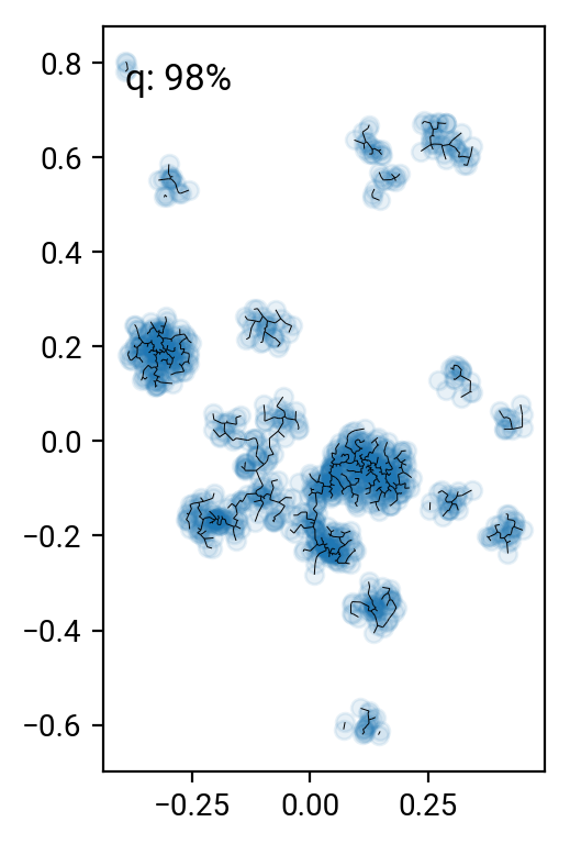
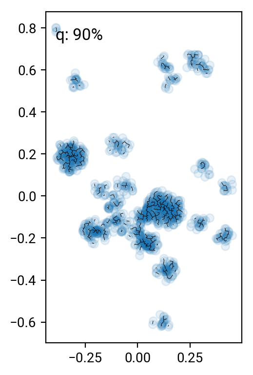
Pruning according to minium distance gives some reasonable results (especially around the 98% cut), but it's pretty hard to come up with a good number that works for all clusters. One can work with alternative distance measures, but they all have their preferred cluster configurations. A nice idea is to go beyond simple distance measures and also identify the connectivity of nodes in the graph. For interested parties, here's the paper by Hong & Dey (2015), where they look at different measures on the graph and find that the number of neighbors of a nodes is a good indicator for that node being in a cluster.

Gap statistic

Finally, if we go back to clustering algorithms that have a fixed cluster number $K$, we'd like to have a way to determine it. Tibshirani, Walther & Hastie (2001) thought of a good one: the Gap statistic. It goes back to the total disperion of the sample with respect to the clusters, which they define as $$W_K(X) = \sum_k^K \frac{1}{2|C_k|}\sum_{i,j\in C_k} d_{ij},$$ i.e. the sum over all in-cluster distances over all clusters. $d$ can be any distance measure, often it's the squared Euclidean $d_{ij} = \lVert x_i - x_j\rVert_2^2$. It's clear that if one increases $K$, this statistic needs to go down, but it's often hard to determine what a good value of it ought to be. So, they simply compare it to the clustering result of a reference distribution without clusters, normally a uniform random distribution over the data volume. In detail, $$\mathrm{Gap}_K(X) = \langle \log W_K\left(X_\mathrm{ref}\right) \rangle - \log W_K(X)$$ The expectation value comes from $B$ clustering runs over independent draws from the reference distribution. Their proposal is to adopt the value $K$ for which $\mathrm{Gap}_K(X) \geq \mathrm{Gap}_{K+1}(X) - s_{K+1}$, where $s$ refers to the standard deviation of $\log W_K\left(X_\mathrm{ref}\right)$. This is quite clever because it works with any sort of clustering algorithm that has a fixed $K$ and tells us when it is capable to reduce the total dispersion more for the actual data than for the reference distribution, in other words when it found another cluster.

Let's try if we can determine the optimal number for K-means in our example data:

def getWK(X, labels, ord=None):
    clusters = np.unique(labels)
    K = clusters.size
    W = 0
    for l in clusters:
        sel = labels == l
        N = sel.sum()
        # TODO: for more general norms, the square isn't correct!
        D = np.sum([np.sum(np.linalg.norm(Xi - X[sel], ord=ord)**2) for Xi in X[sel]])
        W += D/(2*N)
    return W

def getGap(X, method, K, ref_dist, ord=None, B=10):
    N = len(X)
    log_WK = []
    log_WK_ref = []
    for b in range(B):
        cm = method(n_clusters=K)
        labels = cm.fit_predict(X)
        log_WK.append(np.log(getWK(X, labels, ord=ord)))
        ref_sample = ref_dist(N)
        cm = method(n_clusters=K)
        ref_labels = cm.fit_predict(ref_sample)
        log_WK_ref.append(np.log(getWK(ref_sample, ref_labels, ord=ord)))
    l = np.mean(log_WK_ref)
    s = np.std(log_WK_ref) * np.sqrt(1 + 1./B)
    return l - np.mean(log_WK), s

def doGapSweep(X, method, ref_dist, Kmax=10, ord=None, B=10):
    g = []
    s = []
    labels = []
    for iK in range(0,Kmax):
        K = iK+1
        g_, s_ = getGap(X, method, K, ref_dist)
        print (K, g_, s_)
        g.append(g_)
        s.append(s_)
    return range(1,Kmax+1), g, s

def uniform_NDbb(N, D=1, bb=None):
    sample = np.random.uniform(size=(N,D))
    if bb is not None:
        sample = bb[0] + (bb[1]-bb[0])*sample
    return sample

from functools import partial
bb = X.min(axis=0), X.max(axis=0)
N = len(X)
ref_dist = partial(uniform_NDbb, D=X.shape[1], bb=bb)
K, g, s = doGapSweep(X, KMeans, ref_dist, Kmax=30)
plt.errorbar(K,g,yerr=s)

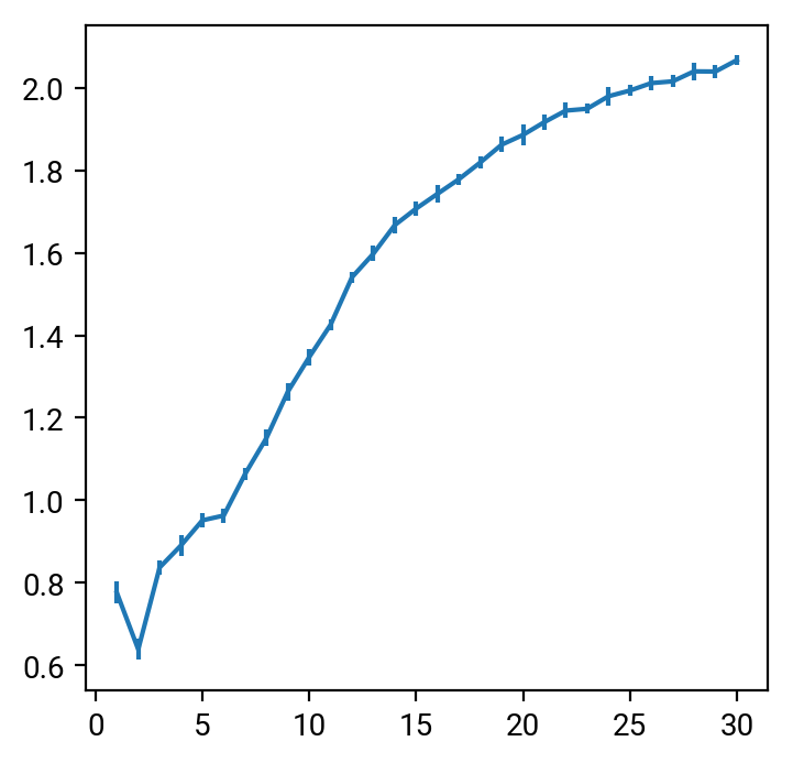
Well, not really. There are a number of caveats for the method, in particular that it doesn't work well for overlapping clusters. The authors mention this limitation themselves, but they don't offer a practical solution. I looked at a few of the pivot points in the graph ($K=3,5,12,21$) and wasn't convinced. Hmm.

Also, for a clustering algorithm that doesn't find a globally optimal solution (most don't), $W_K(X)$ depends on the start configuration. I'd like to replace it (and have done so in the code above) with its expectation value, also obtained from $B$ independent reruns of the sample $X$.

Even then, hmm. On the one hand, I like the idea of comparing against a suitable reference distribution to avoid the guess work, but at some level it must be that the interpretability of the Gap statistic depends on how well the clustering method can deal with the data at hand. I've tried different ones with a couple parameter variations, and they do yield different Gap statistics profiles, but nothing was particularly convincing for our data set.

I consider this another example of a statistics methods that was tested on benign data but doesn't really perform well in a realistic setting. Remember, our data set was strongly clustered by construction.

Extra points for everyone who can tell me how many clusters there really are in the test data...