A basic assumption of many classifications schemes is linear separability (see earlier notes). This assumption will lead to poor classification performance in cases that aren't separable by some hyperplane. A similar problem arises for decision trees and forests when the features don't align well along the coordinate axes of the feature space. 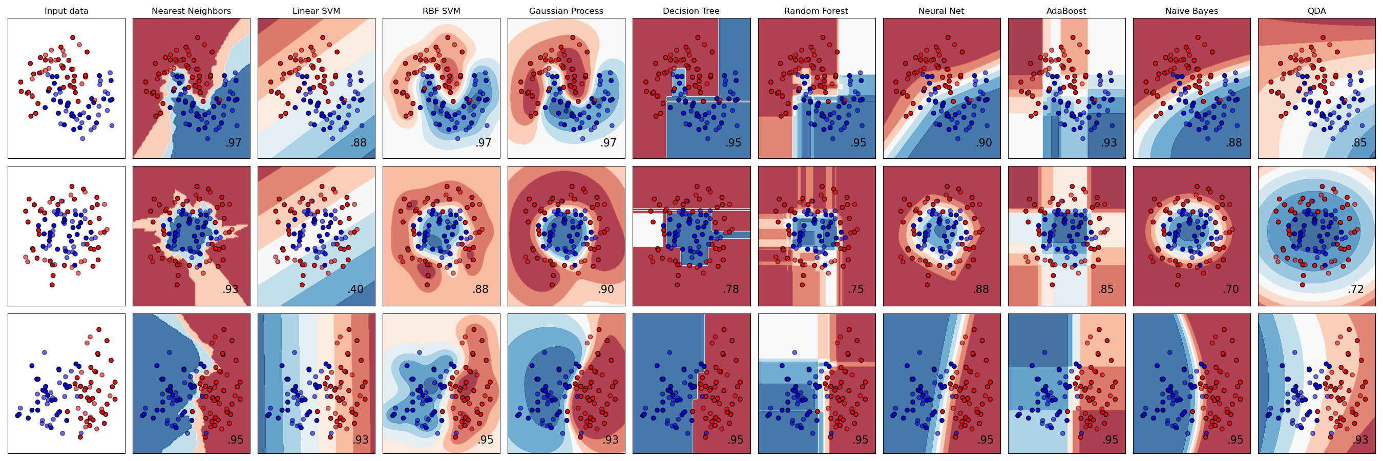The situation becomes quite clear in [this comparison](http://scikit-learn.org/stable/auto_examples/classification/plot_classifier_comparison.html#sphx-glr-auto-examples-classification-plot-classifier-comparison-py) from the scikit-learn website: ![Classifier comparison from scikit-learn](http://scikit-learn.org/stable/_images/sphx_glr_plot_classifier_comparison_001.png) Linear SVM (3rd column) does very well for the linearly separable case (last row), but is really troubled with the Yin-Yang and the inside-outside cases (first and second row). In contrast, trees and forests (6th and 7th columns) present boxy approximations, but generally follow he features quite well. Much smoother approximations can be had from a SVM that uses Radial Basis Functions as kernels (4th column) and neural nets (8th column). The key to both is that they use non-linear transformation of the data, which results in curved decision boundaries. Let's look in detail how neural networks do that. ## Universal approximators It might be strange to look at networks from the perspective of regression since they are mostly used for classifications. But bear with me. When we want to approximate the mapping $X\rightarrow Y$ as observed with $N$ samples $\lbrace x_i,y_i\rbrace, x_i\in\mathbb{R}^D,y_i\in\mathbb{R}$, we first need to account for the dimensionality difference and then for the unknown behavior of the mapping. The first problem can trivially solved by projecting the samples $x $ onto some basis $w$, the second by allowing any function with scalar arguments. Combined this gives us the regression function $\tilde{y}_i = g(w^\top x_i)$, which already provides quite some flexibility. But we can do *a lot* better by using multiple of those regressors and combining them: $$ \tilde{y}_i = \sum_k^K g_k(w_k^\top x_i) $$ It is clear that with $K\rightarrow\infty$ an enormous class of mappings can be approximated, which is why this form is called a **universal approximator**. It is limited, however, to mixtures of scalar functions, but that is really the only restriction. The optimization would have to determine the $w_k$ *and* the functions $g_k$. The concept is known as [projection pursuit regression](https://en.wikipedia.org/wiki/Projection_pursuit_regression), and we will not into details. However, if we now replace the unknown function $g_k$ with a known and fixed function $\sigma$, we get a set of intermediate variables $$ z_k = \sigma(w_k^\top x)\ \text{with}\ w_k\in\mathbb{R}^D\ \ \forall k\in\lbrace1,\dots,K\rbrace $$ This is in fact what the simplest neural network, the single-layer perceptron, does at the beginning. *[For experts: we'll ignore the bias term, which is equivalent to adding a constant 1 as extra feature to the samples. That simply shortens the equations at no loss in generality.]* ```python import numpy as np import matplotlib.pyplot as plt %matplotlib inline plt.style.use('website') import matplotlib matplotlib.rcParams['figure.figsize'] = 3,3 from drawNetwork import * drawNN([5,3], labels=["$X$","$Z$"]) ``` ![png](data-science-in-astronomy-neural-networks-101_files/output_1_0.png) The function $\sigma$ is called **activation function** and there are several typical ones: ```python x = np.linspace(-5,5,101) plt.plot(x,x,label='linear') plt.plot(x,1/(1+np.exp(-x)), label='sigmoid') plt.plot(x,np.tanh(x), label='tanh') plt.plot(x,np.maximum(0,x), label='relu') plt.legend(loc='lower right') ``` ![png](data-science-in-astronomy-neural-networks-101_files/output_3_1.png) It's worth noting that if $\sigma$ is linear, the model is a fancy way of describing a matrix operation, so we're mostly interested in non-linear functions here. There are *some* guidelines which ones to use, but I won't go into those. ## Output layers So far, we've built a single layer with some non-linear transformation and independent weights for each node $z_k$. These are supposed to allow some form of approximation, but of what? This will become clearer when we discuss how we'll complete our simplest network. In the universal approximator above, we simply summed over the transformed variables. That's a fine choice, in particular if the goal of the network is to perform a regression. For more flexibility, we'll allow for weights in that summation: $$ t =\beta^\top z \ \text{with}\ \beta\in\mathbb{R}^K $$ ```python drawNN([5,3,1], labels=["$X$","$Z$","$T$"]) ``` ![png](data-science-in-astronomy-neural-networks-101_files/output_5_0.png) Multivariate regression, i.e. the learning of some mapping $\mathbb{R}^D\rightarrow\mathbb{R}^M$, can be trivially realized with multiple output nodes $$ t_m =\beta_m^\top z \ \text{with}\ \beta_m\in\mathbb{R}^K\ \forall m \in \lbrace1,\dots,M\rbrace $$ ```python drawNN([5,3,2], labels=["$X$","$Z$","$T$"]) ``` ![png](data-science-in-astronomy-neural-networks-101_files/output_7_0.png) But what if we want a classifier? Then, these output simply have to go through another non-linear transformation to ensure that they are bound between 0 and 1 and sum up to 1. One choice is the **softmax** function $$ p_m = \frac{\exp(t_m)}{\sum_l \exp(t_l)} $$ which is the multivariate form of the logit regression we saw earlier in linear classification. The classifier would then choose the class with the maximum $p_m$. Let's look what happened here: we've transformed the original samples $x_i$ in some non-linear fashion, and then run a classifier on the $z_k$ that assumes linear separability. This is quite similar to the kernel trick in SVMs (finding some non-linear mapping to a higher-dimensional space to help with the separability), but with one major difference. The approximator part of the network does not require us to select a kernel function beforehand; instead we pick an activation function, but the weights are determined *from the data*! > A perceptron classifier is a conventional classifier attached to a non-linear approximator, whose parameters are determined from the data Leaves the important question: how are the weigths determined? ## Network training We start by defining a cost function $R=\sum_i R_i$. In the multi-variate regression case, we use the quadratic cost function $$ R_i = \sum_m \left(y_{im} - t_m(x_i)\right)^2. $$ The key to finding the best network weights is to understand that the target values ($t$ or $p$) are **differentiable** functions of the inputs, so we can search for the weights by gradient descent. For the regression case we can write the network equations as $$ t_m(x_i) = \beta_m^\top z(x_i) = \beta_m^\top\left[\sigma(w_1^\top x_i), \dots, \sigma(w_K^\top x_i)\right]\ \forall m \in \lbrace 1,\dots,M\rbrace. $$ which gives $$ \begin{split} &\frac{\partial R_i}{\partial \beta_{ml}}=-2(y_{im}-t_m(x_i))\,z_l(x_i)\equiv \delta_{mi}z_l(x_i)\\ &\frac{\partial R_i}{\partial w_{lj}} = \sum_m^M -2(y_{im}-t_m(x_i))\,\beta_{ml}\, \sigma^\prime(w_l^\top x_i)\, x_{ij} \equiv s_{li} x_{ij} \end{split} $$ For regression the derivation follows the same lines with the cross-entropy $$ R_i = \sum_m y_{im}\log p_m(x_i) $$ as cost function and an extra derivative because of the softmax transformation. As usual, the update equations look like $$ \begin{split} &\beta_{ml}^{\text{it}+1} = \beta_{ml}^{\text{it}} - \gamma^\text{it} \sum_i\frac{\partial R_i}{\partial \beta_{ml}}\\ &w_{lj}^{\text{it}+1} = w_{lj}^{\text{it}}- \gamma^\text{it} \sum_i\frac{\partial R_i}{\partial w_{lj}} \end{split} $$ with a **learning rate** $\gamma>0$. We can now compute these gradients in a two-step process. In the *forward pass*, we fix all weights and compute all $t_m(x_i)$. In the *backward pass*, we compute the current errors $\delta_{mi}$ and propagate them back the the previous layer by $s_{li} = \sigma^\prime(w_l^\top x_i) \sum_m^M\beta_{ml}\delta_{mi}$, which follows directly from the definition of $s_{li}$ above. This scheme, for obvious reasons, it called **back-propagation** and it's the fundamental concept of network training (and the reason why Google's TensorFlow is so good with [automatic differentiation](https://github.com/dfm/tf-tutorial)). ## Photometric redshifts from a simple network We will do a (simplistic) test case of galaxy photometry from 4 different spectral templates, redshifted between 0 and 1, and then observed in 4 different optical filters. ```python # load four template spectra import fitsio path = "data/" templates = [1,3,5,7] seds = {} for k in templates: fp = fitsio.FITS(path+'bpz_%d.sed.fits' % k) seds[k] = fp[1].read() fp.close() plt.semilogy(seds[k]['frequency'], seds[k]['spectral_flux'], label='SED %d' % k) plt.legend(loc='lower left') plt.xlabel('f [THz]') plt.ylabel(r'$f_\nu$') ``` ![png](data-science-in-astronomy-neural-networks-101_files/output_9_1.png) ```python # load the filters bands = ['B','V','R','I'] filters = {} for b in bands: fp = fitsio.FITS(path+'johnson%s.fits' % b) filters[b] = fp[1].read() fp.close() plt.semilogy(filters[b]['frequency'], filters[b]['transmission'], label='Johnson %s' % b) plt.legend(loc='lower left') plt.xlabel('f [THz]') plt.ylabel(r'$T_\nu$') ``` ![png](data-science-in-astronomy-neural-networks-101_files/output_10_1.png) ```python def extrap(x, xp, yp): """np.interp function with linear extrapolation""" y = np.interp(x, xp, yp) y = np.where(x<xp[0], yp[0]+(x-xp[0])*(yp[0]-yp[1])/(xp[0]-xp[1]), y) y = np.where(x>xp[-1], yp[-1]+(x-xp[-1])*(yp[-1]-yp[-2])/(xp[-1]-xp[-2]), y) return y # redshift and apply filters zs = np.linspace(0,1,101) photo = np.empty(len(templates)*len(zs), dtype=[('template','int'),('redshift','float'),('flux','4f')]) i=0 for t in templates: nu_t = seds[t]['frequency'] f_t = seds[t]['spectral_flux'] for z in zs: flux = np.empty(len(bands)) for j in range(len(bands)): b = bands[j] nu_b = filters[b]['frequency'] T_b = filters[b]['transmission'] # shift sed frequency by 1/(1+z) and interpolate at nu_b f_t_z = extrap(-nu_b, -nu_t/(1+z), f_t) # nu decreaseing, need to be increasing for interp/extrap # multiply with filter curve f_t_z_b = f_t_z * T_b # integrate as broadband color flux[j] = f_t_z_b.sum() photo[i] = (t,z,flux) i+=1 for t in templates: mask = photo['template'] == t plt.plot(photo[mask]['redshift'],photo[mask]['flux'][:,0]-photo[mask]['flux'][:,1], label='SED %d' % t) plt.legend(loc='upper right') plt.xlabel('z') plt.ylabel('B-V') ``` ![png](data-science-in-astronomy-neural-networks-101_files/output_11_1.png) Note that the "color" axis is not in magnitudes, but in per-band fluxes, so the typically intuition for what colors mean doesn't apply here. The point is that these templates strongly overlap in some part of the "color"-redshift space. They also overlap in the space of multiple colors: ```python def plotColors(data, scatter=False, legend=True, label=False, ax=None): _templates = np.unique(data['template']) if ax is None: fig = plt.figure() ax = fig.add_subplot(111) for t in _templates: mask = data['template'] == t x = data[mask]['flux'][:,1]-data[mask]['flux'][:,3] # V-I y = data[mask]['flux'][:,0]-data[mask]['flux'][:,1] # B-V if scatter: ax.scatter(x, y, label='SED %d' % t, s=3) else: ax.plot(x, y, label='SED %d' % t) if label: ax.text(x[0], y[0], '$z=0$', size=6, ha='center') ax.text(x[-1], y[-1], '$z=1$', size=6, ha='center') if legend: ax.legend(loc='upper right') ax.set_xlabel('V-I') ax.set_ylabel('B-V') plotColors(photo, label=True) ``` ![png](data-science-in-astronomy-neural-networks-101_files/output_13_0.png) ```python # training samples with some noise def createTrainingData(photo, std=0.02, withhold_template=None): data = photo.copy() data['flux'] *= 1+np.random.normal(scale=std ,size=(len(data),len(bands))) if withhold_template is not None: mask = data['template'] == withhold_template data = data[~mask] return data data = createTrainingData(photo) plotColors(data, scatter=True) ``` ![png](data-science-in-astronomy-neural-networks-101_files/output_14_0.png) We'll now create a perceptron classifier with a single hidden layer that is trained classify the given colors too determine the galaxy template, marginalized over the redshift. It's simpler to interpret visually what the network is capable of. ```python from sklearn.neural_network import MLPClassifier, MLPRegressor from sklearn.preprocessing import StandardScaler # perform template type classification, marginalized over redshift def createTemplateTraining(data): training_templates = np.unique(data['template']) N = len(zs)*len(training_templates) X = np.empty((N,2)) Y = np.empty(N, dtype='int') i = 0 for t in training_templates: mask = data['template'] == t X[i:i+mask.sum(),1] = data[mask]['flux'][:,0]-data[mask]['flux'][:,1] X[i:i+mask.sum(),0] = data[mask]['flux'][:,1]-data[mask]['flux'][:,3] Y[i:i+mask.sum()] = t i += mask.sum() return X,Y # perform redshift regression, marginalized over template def createRedshiftTraining(data): training_templates = np.unique(data['template']) N = len(zs)*len(training_templates) X = np.empty((N,2)) Y = np.empty(N) i = 0 for t in training_templates: mask = data['template'] == t X[i:i+mask.sum(),1] = data[mask]['flux'][:,0]-data[mask]['flux'][:,1] X[i:i+mask.sum(),0] = data[mask]['flux'][:,1]-data[mask]['flux'][:,3] Y[i:i+mask.sum()] = data[mask]['redshift'] i += mask.sum() return X,Y # need to define tab10 for matplotlob < 2.1 (where it's not included as colormap...) from matplotlib.colors import ListedColormap _tab10_data = ( (0.12156862745098039, 0.4666666666666667, 0.7058823529411765 ), (1.0, 0.4980392156862745, 0.054901960784313725), (0.17254901960784313, 0.6274509803921569, 0.17254901960784313 ), (0.8392156862745098, 0.15294117647058825, 0.1568627450980392 ), (0.5803921568627451, 0.403921568627451, 0.7411764705882353 ), (0.5490196078431373, 0.33725490196078434, 0.29411764705882354 ), (0.8901960784313725, 0.4666666666666667, 0.7607843137254902 ), (0.4980392156862745, 0.4980392156862745, 0.4980392156862745 ), (0.7372549019607844, 0.7411764705882353, 0.13333333333333333 ), (0.09019607843137255, 0.7450980392156863, 0.8117647058823529)) cmap_tab10 = ListedColormap(_tab10_data, "tab10") def trainNetwork(data, kind='template', scaler=StandardScaler(), n_nodes=15, alpha=1e-5, plot=True): assert kind in ['template', 'redshift'] if kind == "template": X, Y = createTemplateTraining(data) clf = MLPClassifier(solver='lbfgs', alpha=alpha, hidden_layer_sizes=(n_nodes,), random_state=1) else: X, Y = createRedshiftTraining(data) clf = MLPRegressor(solver='lbfgs', alpha=alpha, hidden_layer_sizes=(n_nodes,), random_state=1) X_ = scaler.fit_transform(X) clf.fit(X_, Y) if plot: h=100 upper = np.max(X, axis=0) * 1.05 lower = np.min(X, axis=0) * 1.05 test_pos = np.meshgrid(np.linspace(lower[0],upper[0],h), np.linspace(lower[1],upper[1],h)) test_pos = np.dstack((test_pos[0].flatten(), test_pos[1].flatten()))[0] test_pos = scaler.transform(test_pos) if kind == "template": pred = np.argmax(clf.predict_proba(test_pos), axis=1) cmap = cmap_tab10 else: pred = clf.predict(test_pos) cmap = 'Spectral_r' pred = pred.reshape(h,h) fig = plt.figure() ax = fig.add_subplot(111) if kind == "template": ax.imshow(pred, cmap=cmap, vmin=0, vmax=10, alpha=0.5, extent=(lower[0], upper[0], lower[1], upper[1]), aspect='auto') if kind == "redshift": c = ax.imshow(pred, cmap=cmap, extent=(lower[0], upper[0], lower[1], upper[1]), aspect='auto') cb = fig.colorbar(c) cb.set_label('redshift') plotColors(data, ax=ax, legend=(kind=="template"), scatter=True, label=(kind=="redshift")) ax.set_title('$n_\mathrm{nodes}=%d$' % n_nodes, size=10) ax.set_xlim(lower[0],upper[0]) ax.set_ylim(lower[1],upper[1]) return clf ``` ```python clf = trainNetwork(data, n_nodes=15) ``` ![png](data-science-in-astronomy-neural-networks-101_files/output_17_0.png) With 15 nodes in the hidden layer, we can see that it did a pretty good job drawing boundaries such that most regions are populated only by the samples of a given template. Note in particular that many of these boundaries are curved and some are inside of others. That's the advantage of the non-linear transformations here. We should, however, keep in mind that we've trained a network with quite a number of weights on just 400 noisy samples. We expect that it's not as good when we train it on some noise samples and then test it on another independent set: ```python X, Y = createTemplateTraining(photo) scaler = StandardScaler() scaler.fit(X) print ("score with perfect data: %.3f" % clf.score(X, Y)) data_ = createTrainingData(photo) X_, Y_ = createTemplateTraining(data_) X_ = scaler.transform(X_) print ("score with noisy data: %.3f" % clf.score(X_, Y_)) ``` score with perfect data: 0.250 score with noisy data: 0.802 And now for the question: how many nodes do we need: ```python for n in [1,5,15,25]: trainNetwork(data, n_nodes=n) ``` ![png](data-science-in-astronomy-neural-networks-101_files/output_21_0.png) ![png](data-science-in-astronomy-neural-networks-101_files/output_21_1.png) ![png](data-science-in-astronomy-neural-networks-101_files/output_21_2.png) ![png](data-science-in-astronomy-neural-networks-101_files/output_21_3.png) As expected, the extent to which the classifier deviates from linear behavior increases with $n_nodes$. It would also increase with the number of hidden layers wedged in between the input and the output layers. As before with the activation function, the number of nodes and hidden layers are configuration parameters for which there are no rigorous guidelines. Experimentation and cross-validation are key. ## NN photo-z estimation We finish this intro with a (silly) regression case. Given a set of colors (two in fact), we ask the network to predict the redshift, ignoring that there are multiple solutions because there are four different spectral templates in the data. ```python clf = trainNetwork(data_, kind='redshift', n_nodes=30) ``` ![png](data-science-in-astronomy-neural-networks-101_files/output_24_1.png) We can see that for the red group (SED 7), it does recognize the difference between the low and high-redshift cases at the top-left of the plot. Similarly, the general behavior of the other types that redshift increases from left to right is well captured. But there are obviously regions with non-sensical estimates of $z<-0.5$. That's because there were no training data to put any penalty on such solutions. In essence, the non-linear nature of the networks means that there can be arbitrary extrapolation errors. It's therefore best to avoid areas with few or no training data. The regression in the central region is tough because different templates go through the same region in color space at different redshifts. Breaking this degenercy is possible but will require more data, more bands, and the hope that we have all possible galaxy types in the training sample. Yeah, photo-zs are hard!

Data Science in Astronomy: Neural networks 101

Date
Mon, 14.05.2018