Data Science in Astronomy: pyTorch introduction
Neural networks without clutter
This post is based on this pyTorch tutorial.
We'll construct a simple network to predict y from x by minimizing squared Euclidean distance. In detail it'll be a fully-connected network with one hidden layer (at first) and a sigmoid activation function. The point of this post is not to build a cutting-edge regression method, but to demonstrate how easy it is to go about it with pyTorch. Let's start by defining a function we like to learn: for something simple but non-linear we'll combine harmonic functions, but throw in a complication, namely that the sampling is densely only in the center. For good measure, we'll also add some noise because nothing is noise-free. To make it easy to visualize, they feature space is two-dimensional, and the output variable is scalar.
import torch

# N is batch size; D_in is input dimension;
# H is hidden dimension; D_out is output dimension.
N, D_in, H, D_out = 1000, 2, 50, 1

# Create test tensors to hold input and output
x = torch.randn(N, D_in) * 3.1415
y = (x[:,0].sin() + x[:,1].cos()).unsqueeze(1)
noise = torch.randn(N, D_out) * 1e-1
y += noise
Let's first have a look at our data:
%matplotlib inline
import matplotlib.pyplot as plt
plt.style.use('website')
plt.scatter(x.numpy()[:,0], x.numpy()[:,1],c=y.numpy()[:])
plt.xlim(-10,10)
plt.ylim(-10,10)

It's a clearly visible deterministic signal with sparse sampling in the outskirts. Now let's design a network to learn the mapping .
This implementation uses the nn package from PyTorch to build the network. PyTorch autograd makes it easy to define computational graphs and take gradients, but raw autograd can be a bit too low-level for defining complex neural networks; this is where the nn package can help. The nn package defines a set of Modules, which you can think of as a neural network layer that has produces output from input and may have some trainable parameters.
# Use the nn package to define a simple model as a sequence of layers.
# Here: Linear / Sigmoid / Linear,
# i.e. a single-layer preceptron with a linear mapping at the end
class TwoLayerNet(torch.nn.Module):
    def __init__(self, D_in, H, D_out):
        """
        In the constructor we instantiate two nn.Linear modules and assign
        them as member variables.
        """
        super(TwoLayerNet, self).__init__()
        self.linear1 = torch.nn.Linear(D_in, H)
        self.linear2 = torch.nn.Linear(H, D_out)

    def forward(self, x):
        """
        In the forward function we accept a Tensor of input data and we
        must return a Tensor of output data. We can use Modules defined
        in the constructor as well as arbitrary operators on Tensors.
        """
        h = self.linear1(x).sigmoid()
        y_pred = self.linear2(h)
        return y_pred
The elegant part in pyTorch (and tensorflow) is that it simply declares how the data x flow through the network: a linear mapping (with a matrix and a bias vector), going from 2 dimensions to 50; a sigmoid transformation, applied element-wise; another linear mapping to go from 50 dimensions to 1. Done.
Because that was such a lot of code to write (:sarcasm:), pyTorch makes it even easier:
# nn.Sequential is a Module which contains other Modules,
# and applies them in sequence to produce its output.
model = torch.nn.Sequential(
    torch.nn.Linear(D_in, H),
    torch.nn.Sigmoid(),
    torch.nn.Linear(H, D_out)
)
In essence, it provides the building blocks for constructing complex mappings with linear and non-linear operations.
To optimize the parameters of this model, here: the matrices and bias vectors of linear1 and linear2, we have to define a loss function. For regression that's the usual Mean Squared Error (MSE) of the predicted value : . It's already coded up in pyTorch, together with several other common ones, e.g. for classification tasks.
And then we do what one always does in convex optimization, namely making steps in the negative gradient direction. This is where tensorflow's automatic differentiation is so useful. Because all transformations are declared in the class TwoLayerNet, the code figures out how to calculate gradients on its own. We only have to do the steps:
# initialize the model
model = TwoLayerNet(D_in, H, D_out)

# The nn package also contains definitions of popular loss functions;
in this case we will use Mean Squared Error (MSE) as our loss function.
loss_fn = torch.nn.MSELoss(reduction='sum')

learning_rate = 1e-4
for t in range(1001):
    # Forward pass: compute predicted y by passing x to the model.
    # Module objects override the __call__ operator so you can call them
    # like functions. When doing so you pass a Tensor of input data to the
    # Module and it produces a Tensor of output data.
    y_pred = model(x)

    # Compute and print loss. We pass Tensors containing the predicted and
    # true values of y, and the loss function returns a Tensor containing
    # the loss.
    loss = loss_fn(y_pred, y)
    if t % 100 == 0:
        print(t, loss.item())

    # Zero the gradients before running the backward pass.
    model.zero_grad()

    # Backward pass: compute gradient of the loss with respect to all the
    # learnable parameters of the model. Internally, the parameters of
    # each Module are stored in Tensors with requires_grad=True, so this
    # call computes gradients for all learnable parameters in the model.
    loss.backward()

    # Update the weights using gradient descent. Each parameter is a
    # Tensor, so we can access its gradients like we did before.
    with torch.no_grad():
        for param in model.parameters():
            param -= learning_rate * param.grad
0 933.7546997070312
100 898.05712890625
200 827.8410034179688
300 703.25537109375
400 613.7958984375
500 529.8275756835938
600 433.88458251953125
700 351.5511169433594
800 291.5534973144531
900 254.2714385986328
1000 231.09042358398438
We have reduced the step sizes by a factor learning_rate, which is supposed to ensure that we can converge even when doing simultaneous downhill gradient steps for multiple optimization parameters may not be a fully stable (or beneficial) thing to do. Let's look at the prediction with a finer resolution:
xt = torch.linspace(-10,10,100)
xt = torch.stack(torch.meshgrid((xt, xt)), dim=2)
yt = model(xt).detach() # need to detach from model for further use

yt = torch.t(yt.squeeze(2))
plt.imshow(yt, extent=(-10,10,-10,10))
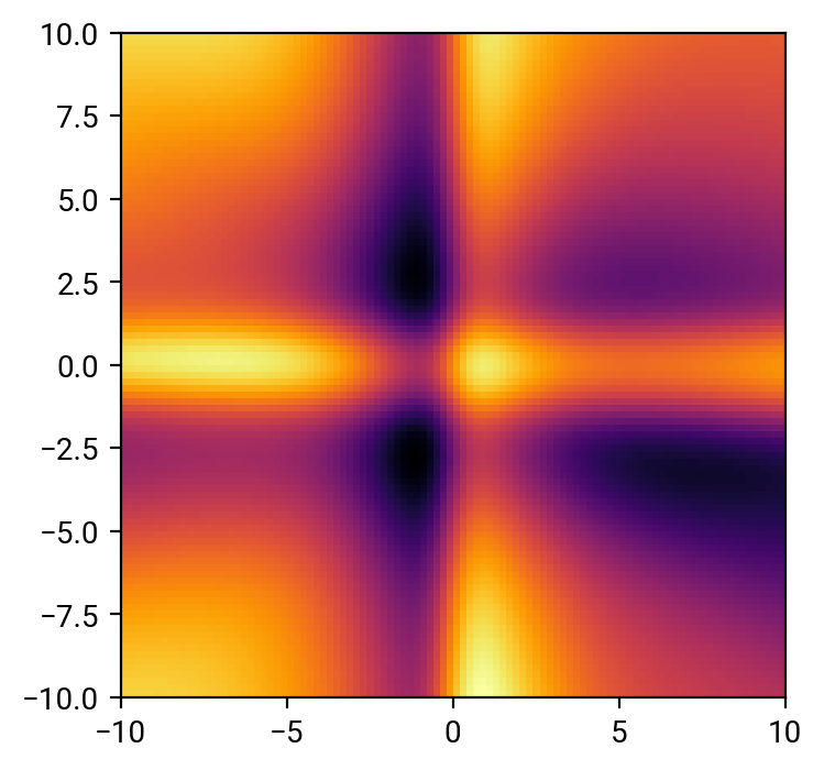
The prediction is quite decent where the sampling of the data is dense, but it get's very shaky in the corners. That's common:
Don't use networks where they have to extrapolate!
Also, depending on the data and the width of the network, a direct optimization can work or sometimes fail quite miserably. This has to do with the loss function not being fully convex in all parameters. In essence, a direct gradient approach may not be ideal. Instead we'll use another optimization method, Adam, that performs a stochastic gradient evaluation and can handle loss functions that occasionally increase.
Again, it's already coded up in pyTorch:
# initialize the model
model = TwoLayerNet(D_in, H, D_out)

# Use the optim package to define an Optimizer that will update the
# weights of the model for us. Here we will use Adam; the optim package
# contains many other optimization algoriths. The first argument to the
# Adam constructor tells the optimizer which Tensors it should update.
learning_rate = 1e-3
optimizer = torch.optim.Adam(model.parameters(), lr=learning_rate)
for t in range(1000):
    # Forward pass: compute predicted y by passing x to the model.
    y_pred = model(x)

    # Compute and print loss.
    loss = loss_fn(y_pred, y)
    if t % 100 == 0:
        print(t, loss.item())

    # Before the backward pass, use the optimizer object to zero all the
    # gradients for the variables it will update (which are the learnable
    # weights of the model). This is because by default, gradients are
    # accumulated in buffers( i.e, not overwritten) whenever .backward()
    # is called. Checkout docs of torch.autograd.backward for details.
    optimizer.zero_grad()

    # Backward pass: compute gradient of the loss with respect to model
    # parameters
    loss.backward()

    # Calling the step function on an Optimizer makes an update to its
    # parameters
    optimizer.step()
0 1078.5792236328125
100 899.9740600585938
200 864.6139526367188
300 800.7428588867188
400 707.2975463867188
500 603.0485229492188
600 510.47747802734375
700 437.02008056640625
800 377.6645812988281
900 329.94488525390625
yt = model(xt).detach()

yt = torch.t(yt.squeeze(2))
plt.imshow(yt, extent=(-10,10,-10,10))

This still may not be overly great, so let's try to make our model more complex by adding another fully connected layer (which adds parameters) and keep going for 2000 steps:
model = torch.nn.Sequential(
    torch.nn.Linear(D_in, H),
    torch.nn.Sigmoid(),
    torch.nn.Linear(H, H),
    torch.nn.Sigmoid(),
    torch.nn.Linear(H, D_out)
)

learning_rate = 1e-3
optimizer = torch.optim.Adam(model.parameters(), lr=learning_rate)
for t in range(2000):
    y_pred = model(x)
    loss = loss_fn(y_pred, y)
    if t % 100 == 0:
        print(t, loss.item())

    optimizer.zero_grad()
    loss.backward()
    optimizer.step()
0 1446.3250732421875
100 914.260009765625
200 898.2183837890625
300 862.9479370117188
400 778.392333984375
500 592.9867553710938
600 402.9549255371094
700 315.80804443359375
800 248.01148986816406
900 208.93670654296875
1000 183.0381317138672
1100 165.38995361328125
1200 151.40463256835938
1300 138.21383666992188
1400 127.8183822631836
1500 118.86930084228516
1600 110.86335754394531
1700 103.80579376220703
1800 97.83943939208984
1900 92.97871398925781
yt = model(xt).detach()

yt = torch.t(yt.squeeze(2))
plt.imshow(yt, extent=(-10,10,-10,10))

Not too bad. And that was done with only a few lines of code, which allows for quick exploration of what works and what doesn't.
My summary:
pyTorch hides the complexity of tensorflow and thereby emphasizes the structure of the network