Gaussian mixture models for Astronomy
An intro for observational data analysis projects
This note is a gentle intro to this paper and the python code pyGMMis.
Gaussian mixture models (GMMs) are to most common kind of mixtures models, and those can be used in plenty of ways. Any process that is additive can be described by mixture models. Think of signal vs background, the measurements of star and galaxy properties, multiple sources contributing to an image.
GMMs have very nice properties that are relevant for observational astronomy: they can deal with noise and incompleteness. Let's see how that works...
GMMs and noise
If we want to fit the probability density function (PDF) of set of data samples with a mixture model, that's what we need to do: maximize the observed likelihood
with respect to the mixing amplitudes and per-component parameters . For GMMs, those parameters are a mean and a covariance matrix . A key problem is that the association of data samples to GMM components is unknown. Otherwise we could simply compute the mean and covariance given all samples associated with any component; the mixing amplitude would then be given by the relative abundance of those samples compared to all data.
One common solution was proposed by Dempster et al. (1977): the Expectation-Maximization procedure. Without going into specifics, the methods amounts to iterations of updates to all involved quantities that provably converge a local minimum of the likelihood. It's not the fastest method, but it works.
Bovy et al. (2011) realized the data samples could be noisy, , with Gaussian errors drawn from independent distributions. This insight is a heteroscedastic extension of the known relation that the PDF of is given by the convolution , which in the case of Gaussian has a width . In essence, if you want to get rid of the error, you need to deconvolve from its PDF, which boils down to subtracting the width of its PDF. That you can do this even when every sample has its own error gave rise to the name Extreme Deconvolution and to the popularity of the method. It can be used for fitting a very wide range of noisy data, or to fit a straight line in 2D when both and values have, potentially independent, errors.
Caveat: For it to properly work, the noise PDFs need to be Gaussian, and the underlying data PDF should be reasonably describable be a GMM with a finite number of components. We will encounter this requirement again later on.
GMMs and incompleteness
What happens if not every sample that was initially generated by the process we seek to model has been observed? This situation is common in observational studies, maybe because a detector isn't (as) sensitive in some areas or because some samples are deemed untrustworthy. Sometimes the nature of the underlying process doesn't allow particular values for data features or combinations thereof.
We're thus faced with another stochastic process, called missingness mechanism by Rubin (1976) or completeness in astronomy, which may not be a fair one. If it isn't, the model will be biased towards the better observed regions in the data because the likelihood, and thus the EM procedure, only cares about observed samples.
Mixture models are unreliable in the regions of unfairly sampled data!
Note: The terminology is sometimes confusing. We might call a situation with missing samples, well, missing data, but that term is used differently in statistics. It refers to a case where some features of a sample may be missing, not the entire sample. The latter case is called truncated data, and a few approaches exist to deal with that. None are as flexible as what I'll introduce with this toy example:
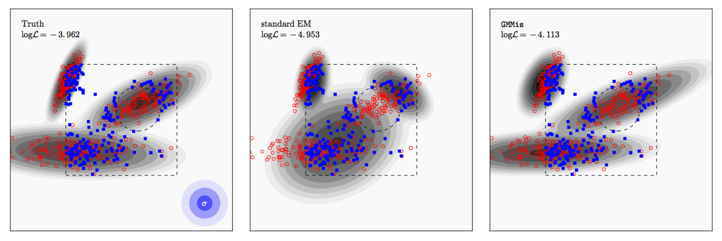
In the example above, the true distribution is shown as contours in the left panel. I then draw 400 samples from it (red), add Gaussian noise to them (1,2,3 sigma contours shown in blue), and select only samples within the box but outside of the circle (blue).
The standard EM algorithm fits the observed samples (blue) only. I don't even attempt to deconvolve from the errors here because this would horribly go wrong since the underlying distribution (after rejecting the samples from the "forbidden" regions, doesn't look like one that can be well fit with three Gaussians.
But there is hope. In Dempster's paper, he already suggest that as part of the EM procedure one can generate mock samples from the current model to augment the observed ones. What I've done in the paper is to work out how do this in practice. At each step the procedure draws samples from the current model, tests which of them should not be observed, and fits those and the observed samples to update the component parameters. This way, the components pull towards the forbidden regions, but always remain hinged to the observed regions. You can see the result in the right panel above, where I also applied the Extreme Deconvolution step.
If you can write down the missingness mechanism, may it be deterministic or stochastic, and if that mechanism does not depend on the underlying PDF, this extension can account for a modest amount of incompleteness. Obviously, if all samples from one component are gone, nothing can be done. In the paper, I've tried to work out what that limit is, and came up with . In words: the number of observed samples of component compared to all observed samples should exceed the average mixing fraction. This is quite restrictive, and goes is caused by the "greedy" nature of the EM procedure. If a component is not expressed much, there's not a lot of reason to even bother to fit it. In fact, the failure mode of this new procedure is not a bad fit of poorly expressed components, but their complete absence from the fit.
Two note on cases with noise and incompleteness, like the example above:
- The mock samples need to be noisy, too. This means you need to be able to write down another process, namely the one that sets the errors for each sample. That's trivial if the errors are i.i.d, but may require extra work if the errors are variable.
- Adding noise and rejecting samples do not commute. The procedure works in both cases, as long as the internal representation of the missing samples complement the observed ones to give an approximation of the completely observed data.
Background vs Signal
As I said above, mixture model are really useful. We can perform a two-level fit, where to top level decides if a sample belongs to signal or background, and the next level fits a GMM to the signal portion:
How can we know which samples belong to the signal? We again ask the model. Effectively, we exclude all samples that have a higher probability under the background model than under the signal GMM model. This decision is stochastic so that the algorithm can explore the boundary between the two components, but again we can deploy the EM procedure to our advantage.
Now we have all we need for the application in the paper: modeling the X-ray luminosity of the galaxy NGC 4636. The data come from then Chandra ACIS-I instrument in the 0.5-2 keV band, and have a few relevant characteristics:
- X-ray photons are recorded individually, not binned into pixels like most imagers do.
- The detector doesn't fairly observe the sky: it has chip gaps and sensitivity variations.
- Most of the photons come from compact point sources, while we're interested in the diffuse emission of the galaxy. We could model them as well, but it's faster to mask them. Another selection effect.
- ACIS-I has a point spread function that is very well approximated by a Gaussian, but its width spatially varies by a factor of 30. Because the PSF is equivalent to an additive error on the photon positions, we want to deconvolve on the fly.
- There's a faint but noticeable X-ray background that is approximately spatially uniform. We can model this as well while we're at it.
The data set comprises 150k photons, and I fit it with 60 components. The runtime is a few minutes on my laptop. Here's the result:

Top left is the data, after some calibration steps, top right the completeness from the detector sensitivity and the extra masks we added to remove point sources. Bottom left is the "internal" view of the scene: the method's preception of the complete observation, including the background but without the point sources that we didn't want to model. Because we mask them entirely, they become intentionally irrecoverable. Bottom right is the model of the signal portion: the diffuse emission of NGC 4636.
Conclusion
The GMM is incredibly useful for many applications. So is the EM procedure. Combining both allows us not only to fit a wide range of data, but to remove the noise, and to fill in samples that were missing.
But there is no such thing as a free lunch:
- For a sensible fit, the underlying data PDF should be describable by a GMM, i.e. a finite number of Gaussians.
- If you want to account for incomplete sampling, you're at the mercy of the GMM assumption. If it's valid, the mock samples will do a fine job.
- If you want to deconvolve from the errors, they have to be Gaussian, too. And you have to known them.
- If you want to deal with incompleteness and noise, the stakes are high, i.e. everything better be Gaussian. In addition, you not only need to know the errors, but be able to predict them for generating proper mock samples that correspond to the observed noisy scene.
I hope this provides some guidance for your data analysis projects. For more details on the code, please have a look at its README.